Classifier-Free Guidance
Introduction
Classifier-free guidance is a technique for improving the quality of generated samples from generative models. It has become a staple in diffusion models and flow matching for conditional generation that it is almost always used. This post takes a deep dive into the topic giving a visual explainer and at the same time trying to answer questions like: why do we run the model twice? is it just temperature tuning? and when should we not use it?
 Figure: CFG vector field showing how guidance steers the trajectory toward the conditional distribution.
Background
Diffusion Models / Flow Matching
Both diffusion models and flow matching can be interpreted as utilizing the Langevin dynamics, specifically the Metropolis-adjusted Langevin algorithm (MALA), to sample from the target distribution. MALA is given by the following equation:
\[x_{t+1} = x_t + \alpha_t \nabla_x \log p(x_t) + \mathcal{N}(0, \epsilon_t^2) \tag{1}\]where $x_t$ is the sample at time $t$, $\nabla_x \log p(x_t)$ is the gradient of the log-likelihood of the target distribution, $\alpha_t$ is the step size, and $\mathcal{N}(0, \epsilon_t^2)$ is the noise added to the sample.
 Figure 1: Unconditional generation from a Flow Matching model
While diffusion models learn to predict the score function, i.e. one component of $\nabla_x \log p(x_t)$, flow matching learns to predict the velocity field itself, i.e. $v_t = x_{t+1} - x_{t}$. The diffusion models are learning to denoise the noisy sample, while flow matching learns the linear interpolation between the current sample and the next one.
For simplicity, we will assume a flow matching model for the rest of the post.

Figure 2: (a) A single forward pass through the model takes noisy input x_t and timestep t, producing a velocity/score prediction. (b) Iterative sampling follows these velocity predictions step-by-step from noise distribution to data distribution. (c) The model learns a vector field that transports samples from a Gaussian distribution $\mathcal{N}(0, 1)$ to the target distribution $p(\mathbf{x})$
Classifier Guided Generation
A natural design choice is to train the generative model on the entire dataset unconditionally and then use a classifier to guide the sampling process. However, this approach has two major drawbacks:
- The mode-collapse: an unconditionally trained model may not be able to capture the low density regions, areas with fewer training samples, of the target distribution well.
- Gradient issues: guidance takes the form of:
where $p(x_{t})$ is the unconditional distribution, $\lambda$ is a hyperparameter that controls the strength of the guidance and $p(c \mid x_t)$ is the conditional distribution coming from a classifier.
First, the classifier should have learned a good representation of the condition such that the gradient of the conditional distribution is usable for the sampling process. Second, the difficulty lies combining the gradients effectively by tuning $\lambda$ during inference 1.
Conditional Generation
So far, we have only seen the unconditional generation case. Conditioning is the process of guiding the sampling process towards a specific region of the target distribution and can be fed to the model via class label, text prompt, or other information.

Figure 3: (a) Single forward pass with conditional information c added to the model inputs. The velocity output now depends on both the noisy sample x_t, timestep t, and condition c. (b) Conditional sampling where c = left eye guides the trajectory specifically toward the left eye region of the target distribution.
1 also noted that the classifier-guided generation can still be helpful for an conditionally trained model, even outperforming without guidance as well as unconditionally trained models with classifier guidance. The sampling now utilizes:
\[\nabla_x \log p(x_t \mid c) + \lambda \nabla_x \log p(c \mid x_t)\]where $p(x_t \mid c)$ is the conditional distribution learned by the generative model.
Though the two terms look similar, it is not well understood why this is exactly beneficial. But the difficulty still remains in combining the gradients effectively by tuning $\lambda$ during inference. This is where classifier-free guidance comes in.
WIP ---
Classifier-Free Guidance
The key insight is to make the model learn both the conditional and unconditional distributions during training.
Derivation
This subsection derives the classifier-free guidance formula using the neat Bayesian trick proposed in 2.
\[\log p(x_t | c) + \log p(c) = \log p(c | x_t) + \log p(x_t)\]$p(c)$ term moved to the right side of the equation
\[\log p(x_t | c) = \log p(c | x_t) + \log p(x_t) - \log p(c)\]Taking the gradient with respect to $x_t$:
\[\nabla_{x_t} \log p(x_t | c) = \nabla_{x_t} \log p(c | x_t) + \nabla_{x_t} \log p(x_t)\]Moving $p(x_t)$ term to the left side of the equation:
\[\nabla_{x_t} \log p(x_t | c) - \nabla_{x_t} \log p(x_t) = \nabla_{x_t} \log p(c | x_t) \tag{3}\]The right hand side of equation (3) is the gradient of the conditional distribution of the class label given the sample learned through a classifier in equation (2). Plugging left hand side of equation (3) into equation (2) gives:
\[\nabla_x \log p(x_t, c) = \nabla_x \log p(x_t) + \lambda (\nabla_{x_t} \log p(x_t | c) - \nabla_{x_t} \log p(x_t)) \tag{4}\]Remember that our flow matching model predicts the velocity field: \(v_{t} \propto \nabla_{x_t} \log p(x_t)\).
So we can rewrite equation (4) as:
\[v_{cfg} = v_{u} + \lambda (v_{c} - v_{u})\]where $v_{u}$ is the unconditional velocity, and $v_{c}$ is the conditional velocity. The guidance scale $\lambda$ is a hyperparameter that controls the strength of the guidance. A higher guidance scale will produce more class-specific samples.
We have now rid ourselves of having to use an external classifier. However the question still remains: how do we get both the unconditional and conditional velocity fields? The anwer is to make the same model learn both the unconditional $v_u$ and conditional $v_c$ velocity fields during training. The model is fed with the class labels to learn the conditional velocity field and a null label to learn the unconditional velocity field.
Implementation
The training function is as follows:
def train_step(model: torch.nn.Module,
          x: torch.Tensor,
          labels: torch.Tensor,
          t: torch.Tensor,
          v_target: torch.Tensor,
          null_label: torch.Tensor = torch.tensor(-1.0),
          label_dropout: float = 0.2) -> torch.Tensor:
    """
    Args:
        model: The model to use for training.
        x: The input tensor.
        y: The class tensor.
        v_target: The target velocity tensor.
        null_label: The null label used during training.
        label_dropout: The probability of dropping the label.
    """
    dropout_mask = np.random.rand(x.shape[0]) < label_dropout
    labels[dropout_mask] = null_label # randomly set labels to -1 (unconditional)

    t = np.random.rand(x.shape[0], 1) # Sample random time t ∈ [0, 1]
    x0 = np.random.randn(x.shape[0], 2) # Sample noise
    x_t = (1 - t) * x0 + t * x # Straight-line interpolation
    v_target = x - x0 # Target velocity
    v_pred = model(x_t, t, labels) # Forward pass
    loss = np.mean((v_pred - v_target) ** 2) # Compute MSE loss
    return loss
Once trained, the model can be used to generate samples conditionally as well as unconditionally. The inference function which then utilizes the classifier-free guidance formula is as follows:
def inference_step(model: torch.nn.Module,
                            x: torch.Tensor,
                            labels: torch.Tensor,
                            t: torch.Tensor,
                            null_label: torch.Tensor = torch.tensor(-1.0),
                            cfg_scale: float = 2.0) -> torch.Tensor:
    """
    Args:
        model: The model to use for generation.
        x: The input tensor.
        labels: The class tensor.
        t: The time tensor.
        null_label: The null label used during training.
        cfg_scale: The guidance scale.

    Returns:
        The guided sample.
    """
    v_u = model(x, t, null_label) # Unconditional velocity
    v_c = model(x, t, labels) # Conditional velocity
    v = v_u + cfg_scale * (v_c - v_u) # CFG
    x = x + v * dt # Euler step
    return x
Visualizations
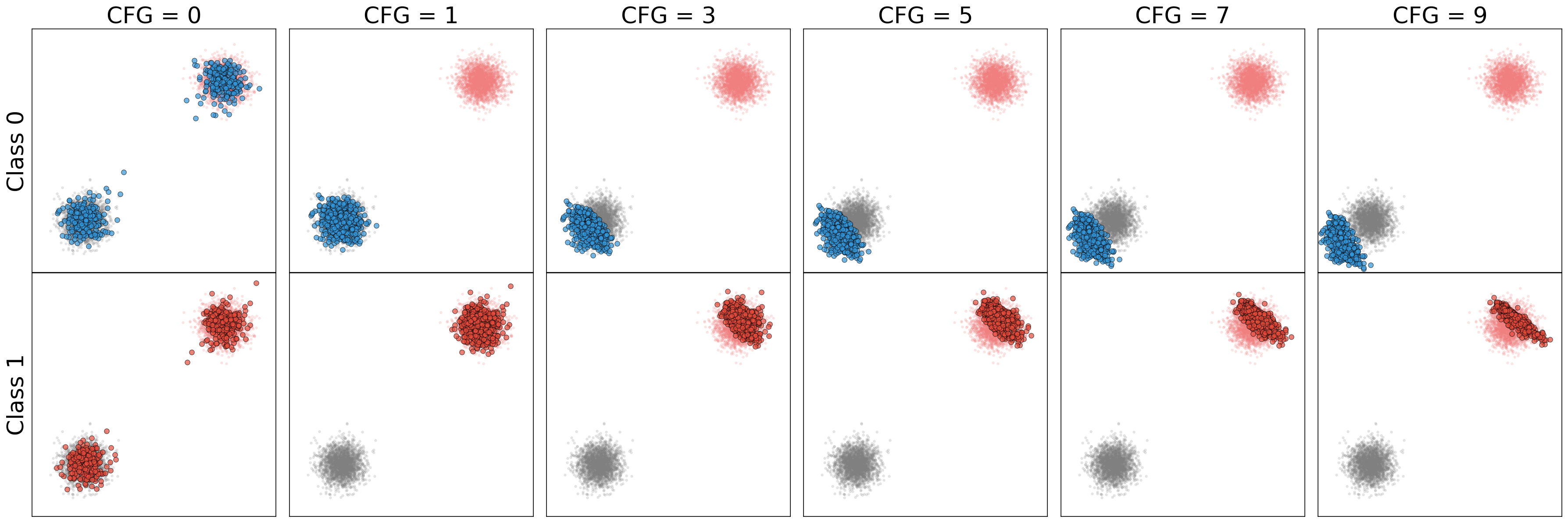 Figure 4: Non overlapping classes: CFG comparison for both classes side by side.
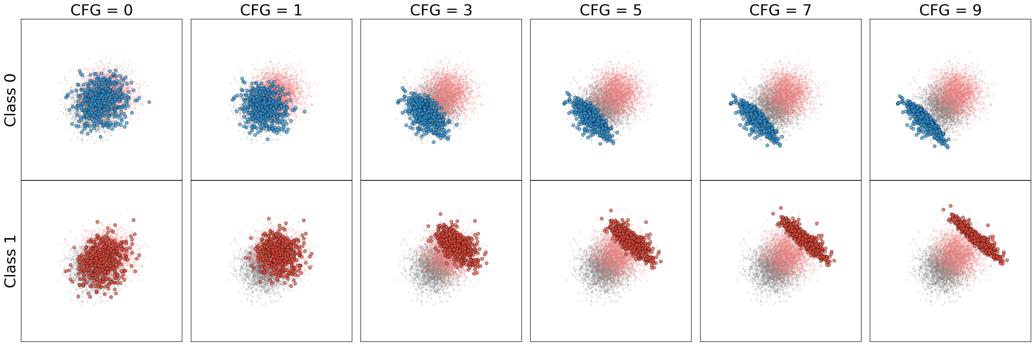 Figure 5: Overlapping classes: CFG comparison for both classes side by side.
 Figure 6: Non overlapping classes: Probability path for both classes side by side.
 Figure 7: Overlapping classes: Probability path for both classes side by side.
Temperature Tuning
Is classifier-free guidance a form of temperature tuning? The answer is yes and no.
Yes, because the guidance scale $\text{cfg_scale}$ > $1.0$ can be interpreted as a way to reduce the temperature of the sampling process. No, because the outcome is a condensation of the distribution towards the class label. It is not a simple temperature reduction. Decreasing the $\text{cfg_scale}$ will not always result in a sharper distribution. In fact, it will result in a more blurred distribution.
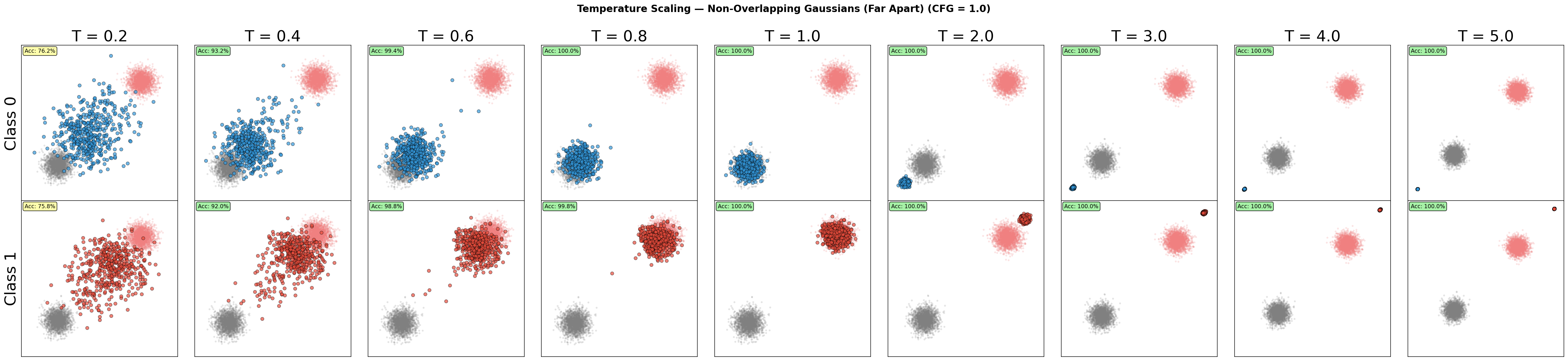 Figure: Temperature scaling for non-overlapping classes.
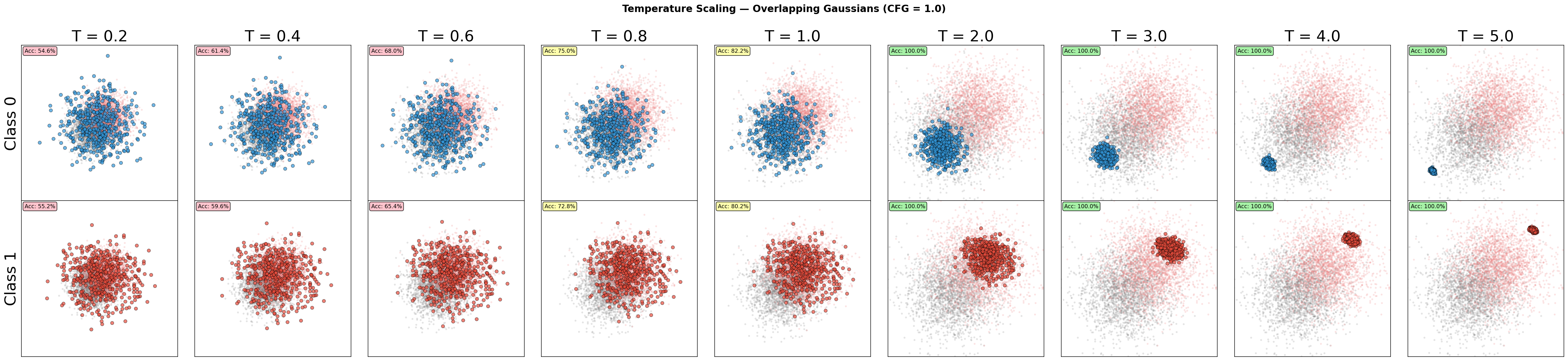 Figure: Temperature scaling for overlapping classes.
Rectified Flow vs Classifier-Free Guidance
Rectified flow is another staple in the generative model toolkit. It is a way to straighten the trajectory of the sampling process, thereby achieving better sampling quality in fewer steps.
 Figure 8: Rectified flow trajectory curvature.
This elegant solution is at odds with the classifier-free guidance.
Rectified CFG
Non-overlapping Classes
 Figure: Rectified CFG trajectory for non-overlapping classes.
 Figure: Rectified CFG probability path for non-overlapping classes.
Overlapping Classes
 Figure: Rectified CFG trajectory for overlapping classes.
 Figure: Rectified CFG probability path for overlapping classes.
Distillation Guidance
Non-overlapping Classes
 Figure: Distillation guidance trajectory for non-overlapping classes.
 Figure: Distillation guidance probability path for non-overlapping classes.
Overlapping Classes
 Figure: Distillation guidance trajectory for overlapping classes.
 Figure: Distillation guidance probability path for overlapping classes.
References
-
Dhariwal, Prafulla, and Alexander Nichol. “Diffusion models beat gans on image synthesis.” In Advances in Neural Information Processing Systems 34 (2021): 8780-8794. ↩ ↩2
-
Ho, J. and Salimans, T. “Classifier-Free Diffusion Guidance.” In Advances in Neural Information Processing Systems (pp. 1-13). 2021. ↩